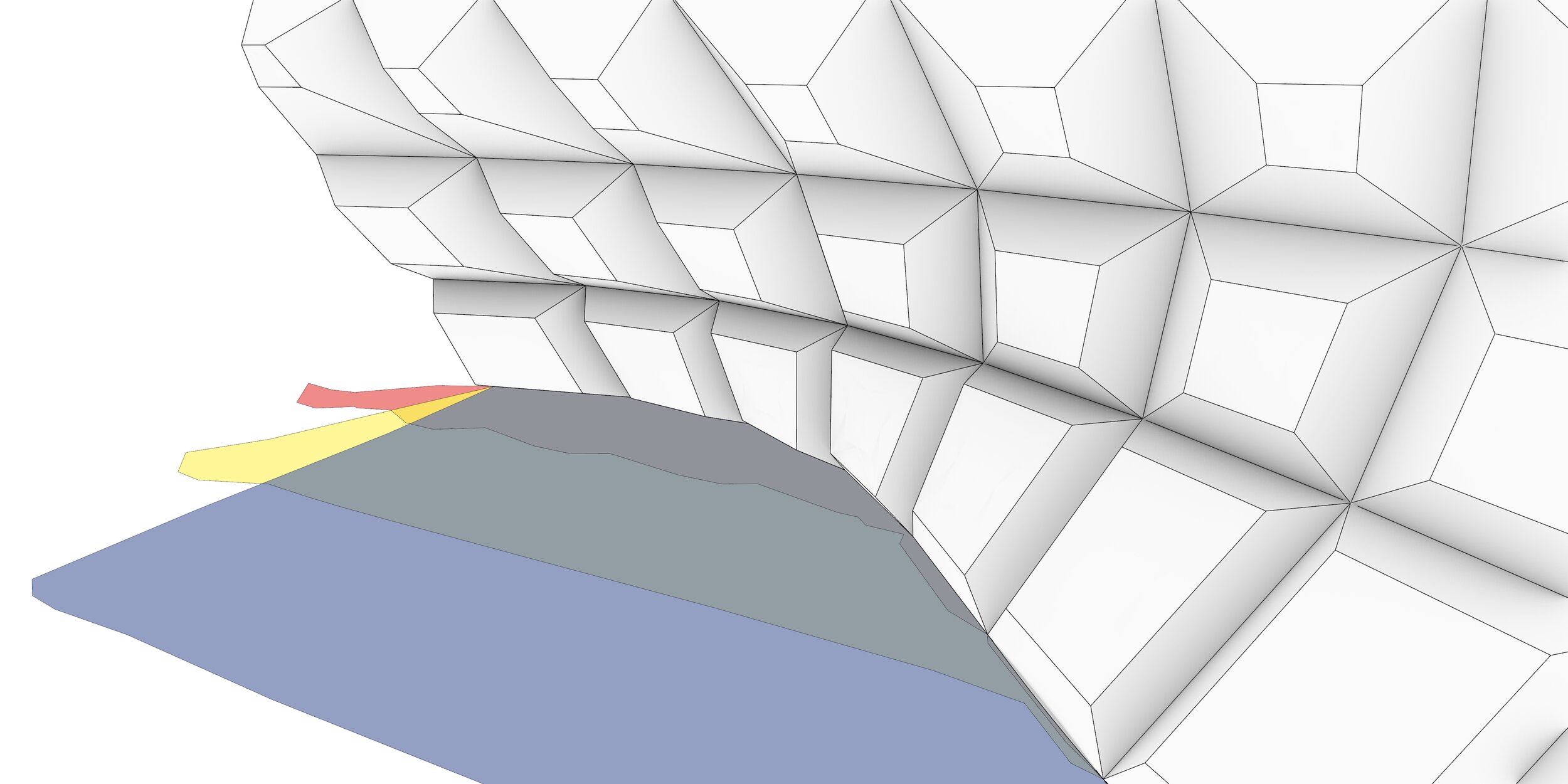
Ladybug Shadow Analysis
This post explores shadow analysis using the Ladybug plug-in for GH.
I’m using Rhino 6 and the model units are in mm. To visualise the outcome I’ve also used the Human plug-in.
*Step 04B is optional and requires the GH Python plug-in which can be obtained from the link below:
Step 00:
Place Ladybug’s Ladybug component before starting the script. If the component is running, it should generate a message similar to this:
Hi smalek! Ladybug is Flying! Vviiiiiiizzz...
Default path is set to: c:\ladybug\
Step 01:
Ladybug plug-in uses weather data to run the analysis. The data can be accessed from various sites. The first option (top) uses Ladybug Tools website. simply select one of the data sources and paste in in a Panel component. Then feed it to Open EPW And STAT Weather Files component.
The second option is to download the EPW file onto your PC and use the Open EPW Weather File component.
I personally prefer the first method as it does not require any files on your PC which means the script can be used on all computers. The second method requires you to save the file with the GH file so it access it on other computers.
Step 02:
The EPW file is then fed to the Import EPW component. This component breaks the data into multiple categories.
One of the most important outputs is modelYear. The more years the EPW covers, the more accurate our analysis will be.
Step 02b*:
The text from of the modelYear output has extra information that are not useful to me so I used the following components to remove the text that is not needed and get rid of duplicate years:
Separate data > Create Set > Sort List
I then turn these components into a Cluster and rename it to Data Year*
Step 03:
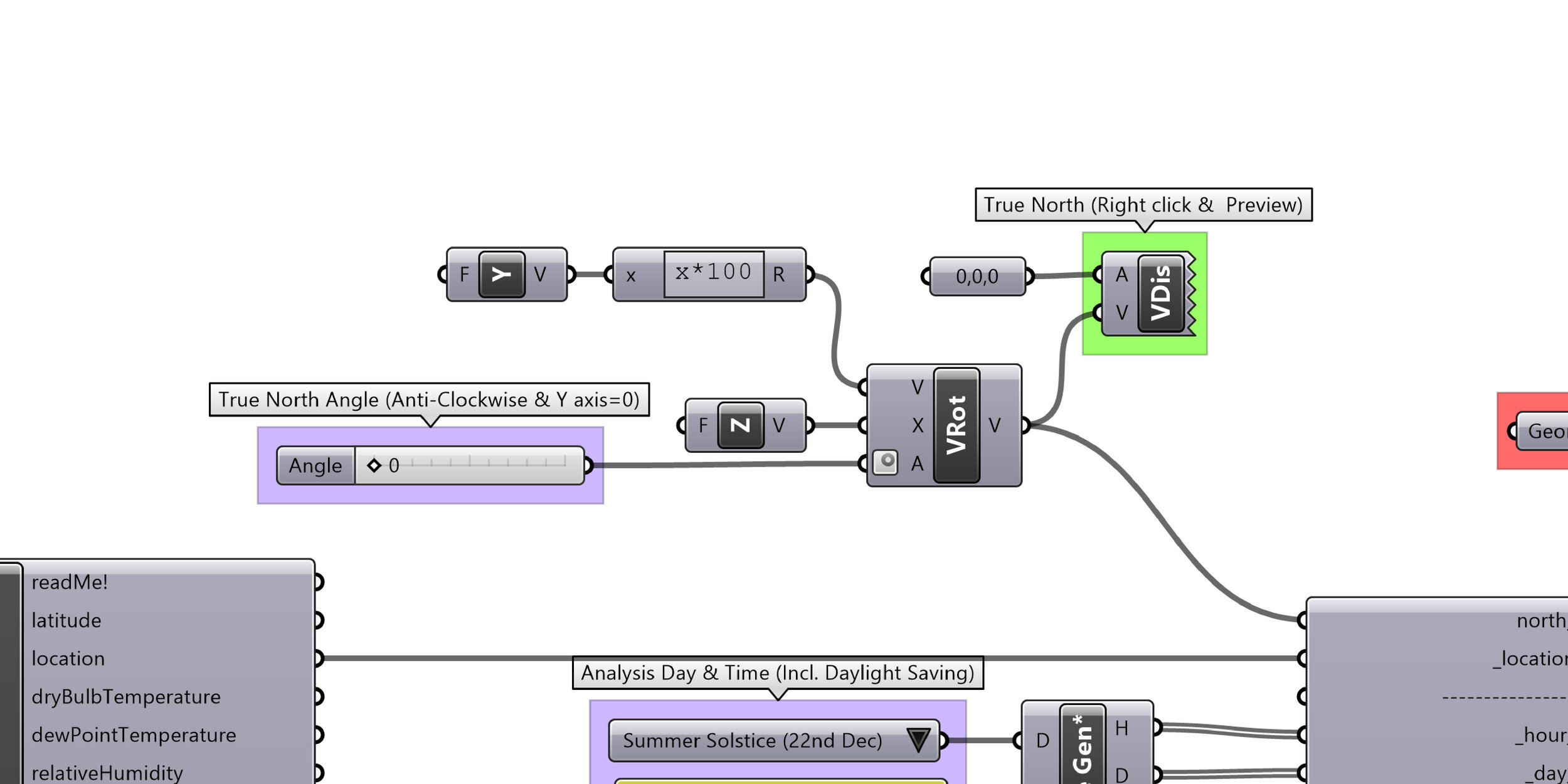
True north is yet on the Y axis. To add more control to the script, I’ve used the following components:
Unit Z > Unit Y > Rotate (VRot) > Vector Display
Step 04:
To set the period of time for the analysis we could use the Analysis Period component. This component allows us to set the months, days and hours of the analysis. The longer the period, the slower the script will be.
This method is the simplest way of setting the analysis period. To add more control over the analysis I use the personalised method below.
Step 04b*:
In the majority of shadow analyses, the time is set on one of the following dates:
Spring Equinox (22nd Sep) = 9
Summer Solstice (22nd Dec) = 12
Autumn Equinox (22nd Mar) = 3
Winter Solstice (22nd Jun) = 6
Step 04c*:
Another crucial factor in the analysis is the daylight saving which makes a huge difference to the outcome. The Date Gen* cluster shown in the previous step is comprised of the following components in response to this problem:
Timer > Time > Split Text > List Item
Python (_Daylight Saving) > Addition
Construct Date > Deconstruct Date
The Python component contains the following lines of code:
"""In Dec & Mar roll back the time by 1 hour"""
if x==12 or x==3:
    a=-1
else:
    a=0
Step 05:
All of previous steps feed into the SunPath component. Other parameters such as sunPathScale and sunScale can also be set from here. The sun path can be baked into Rhino by using a Button component which gets connected to bakeit input.
Step 06:
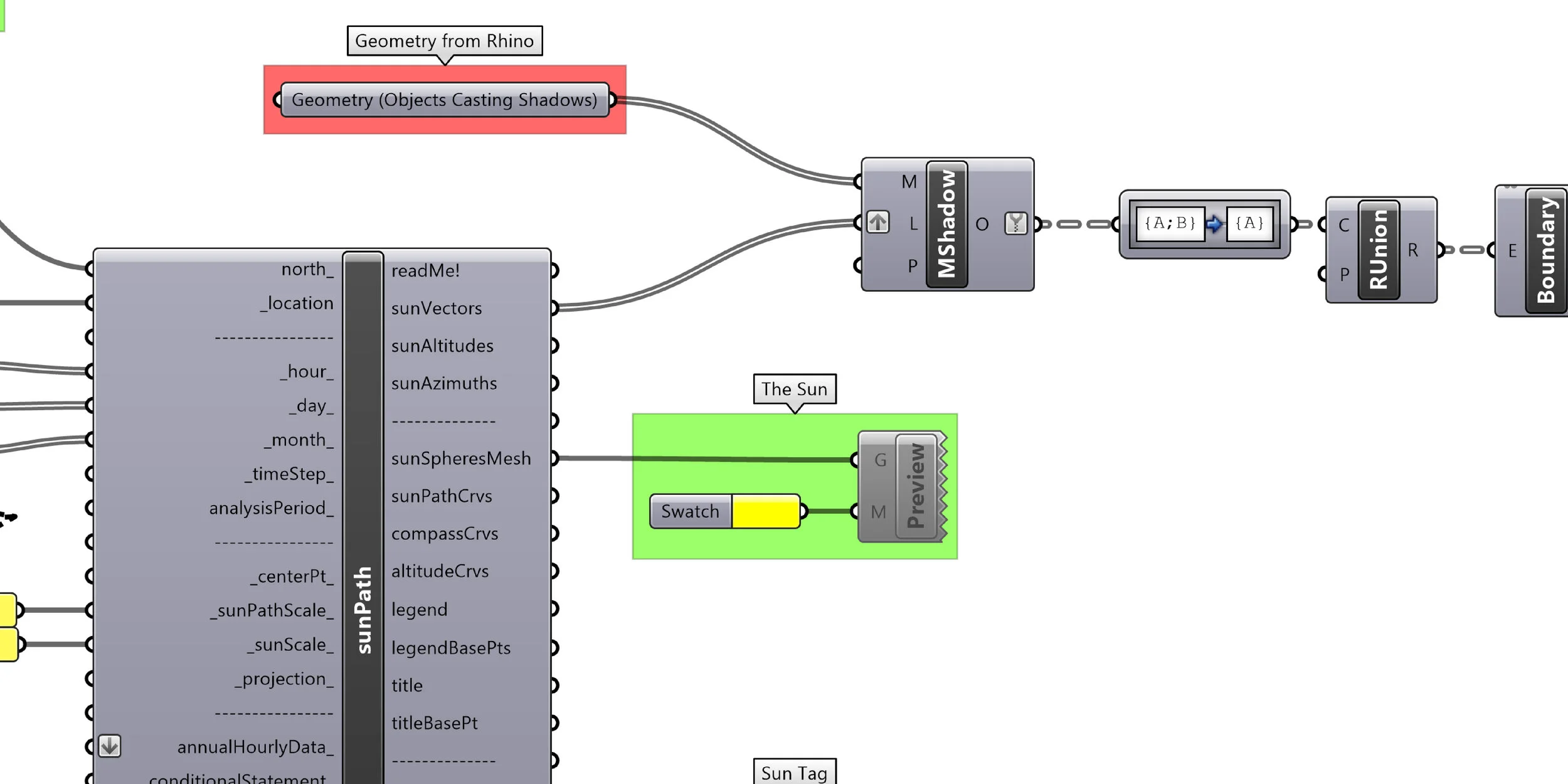
The shadows are generated using the Mesh Shadow component. The geometry from Rhino are connected to the M input and the SunVectors from the SunPath component are connected to the L input. Make sure the L input is grafted. This is crucial for studies covering more than one point in time.
Step 07:
The output of the Mesh Shadow component is for every single object at a time. To merge the shadows of all objects together I’ve used the following components:
Path Mapper > Region Union > Boundary Surface
To edit the Path Mapper, first right click and set it Null Mapping and then double click to make adjustments.
Step 08:
I’ve use a combination of components to generate as many colours as the times of our analysis period. Then we can use Human’s Custom Preview Line Weight and Custom Preview Material to visualise the outcome.
The process of creating colours are covered in more detail in Step 1 and 1B of MetaBall Part 02 post.
To bake the shadows with colours refer to MetaBall Part 03 post.


