Image to Contour
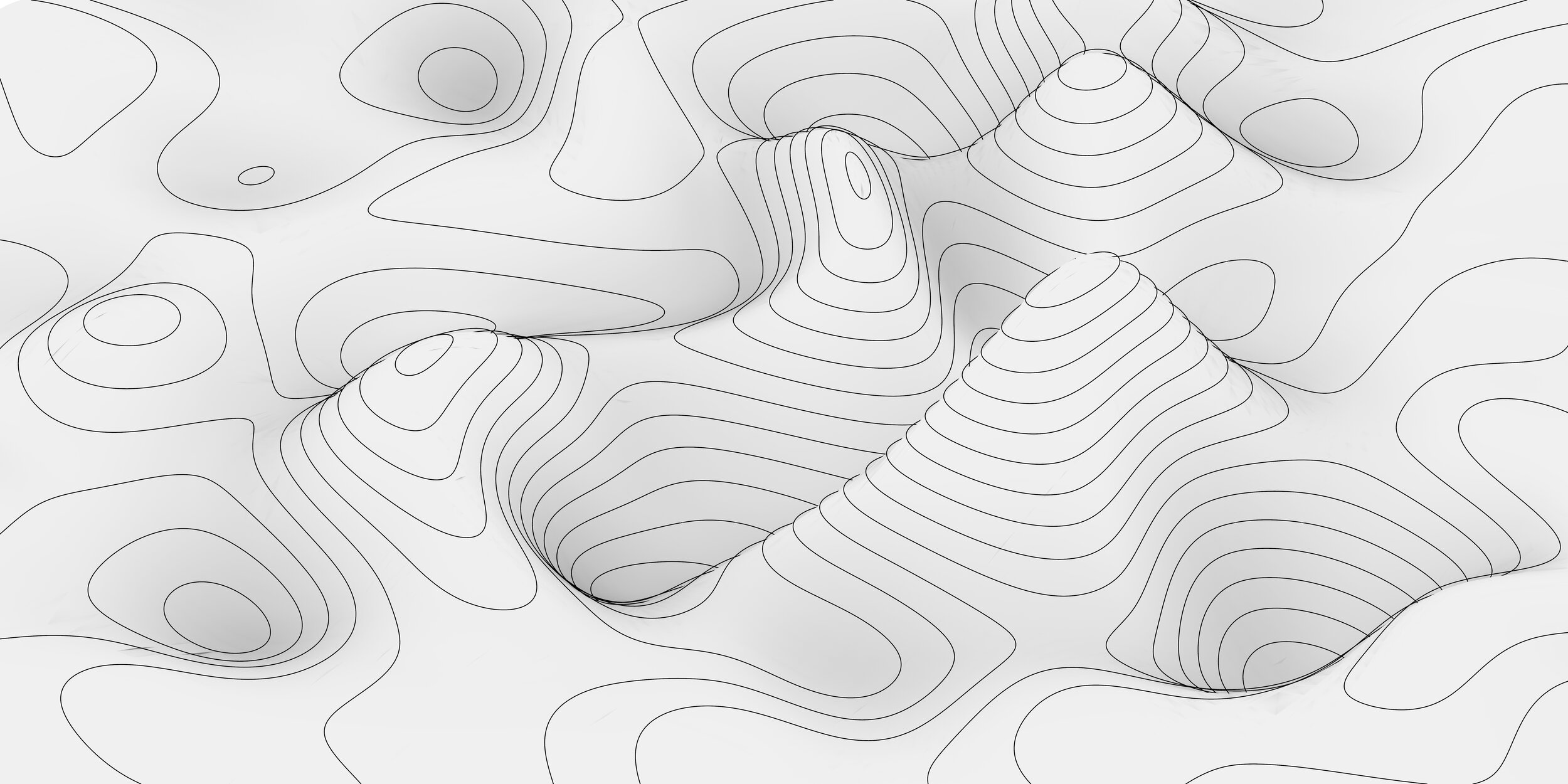
The outcome of this excersize is similar to the Heightfield command in Rhino.
Image to Contour does not require any additional plug-ins for GH. I’m using Rhino 6 and the model units are in mm.
Step 00:
The script is based on a quad shaped polyline. In this example I’ve used the Rectangle component with equal sides which turns the curve into a square.
Then the outcome is connected to a Surface Divide component to place a grid of points inside the square curve.
Tip #1: The number of divisions fed to the Surface Divide component determine the complexity of the surface and the final outcome. The larger the number, the slower the script will be.
Tip #2: Although the outcome of the Rectangle component is a planar curve, the Surface Divide component is smart enough to turn the planar curve into a planar surface and then run the division on it.
Step 01:
The Image Sampler as the name suggests allows us to generate a series of values by sampling an image at certain points. To cross reference the image to our surface and grid of points we feed the UV output of Surface Divide component.
Tip #3: Double clicking on the Image Sampler component allows us to specify the sampled image as well as what to sample for. In this example I’ve used the Colour Brightness (B/W) option.
The outcome of the Image Sampler is not necessarily in a range that would be useful for our purposes. As a result I’ve used a combination of the following components to adjust the numbers:
Bounds > Remap Numbers > Construct Domain
Step 02:
The next step is going to displace the grid of points we created earlier by moving them away from the surface. So we use a Move component and connect the grid of points to the G input.
Similar to Rhino, the next step is to specify a direction and amount for the points to be moved. For the direction I’ve used the N output of the Surface Divide component. The output is a series of vectors perpendicular to the surface and pointing away from it.
Using the Amplitude component we multiply the length of the vectors by the numbers generated by the Image Sampler component.
Tip #4: The reason I used the N (Normal) vectors and not use a Z vector is that it allows the script to be used for surfaces that are not drawn on the XY plane. If a surface was drawn on say YZ plane, the correct vector to use would be the X vector. This is also true if the original surface is curved an not flat.
Step 03:
The next step is to turn the grid of points back into a surface. I’ve done so using the Interpolate (IntCrv) and Loft components. Make sure the C input of the Loft component is Flattened.
Step 04:
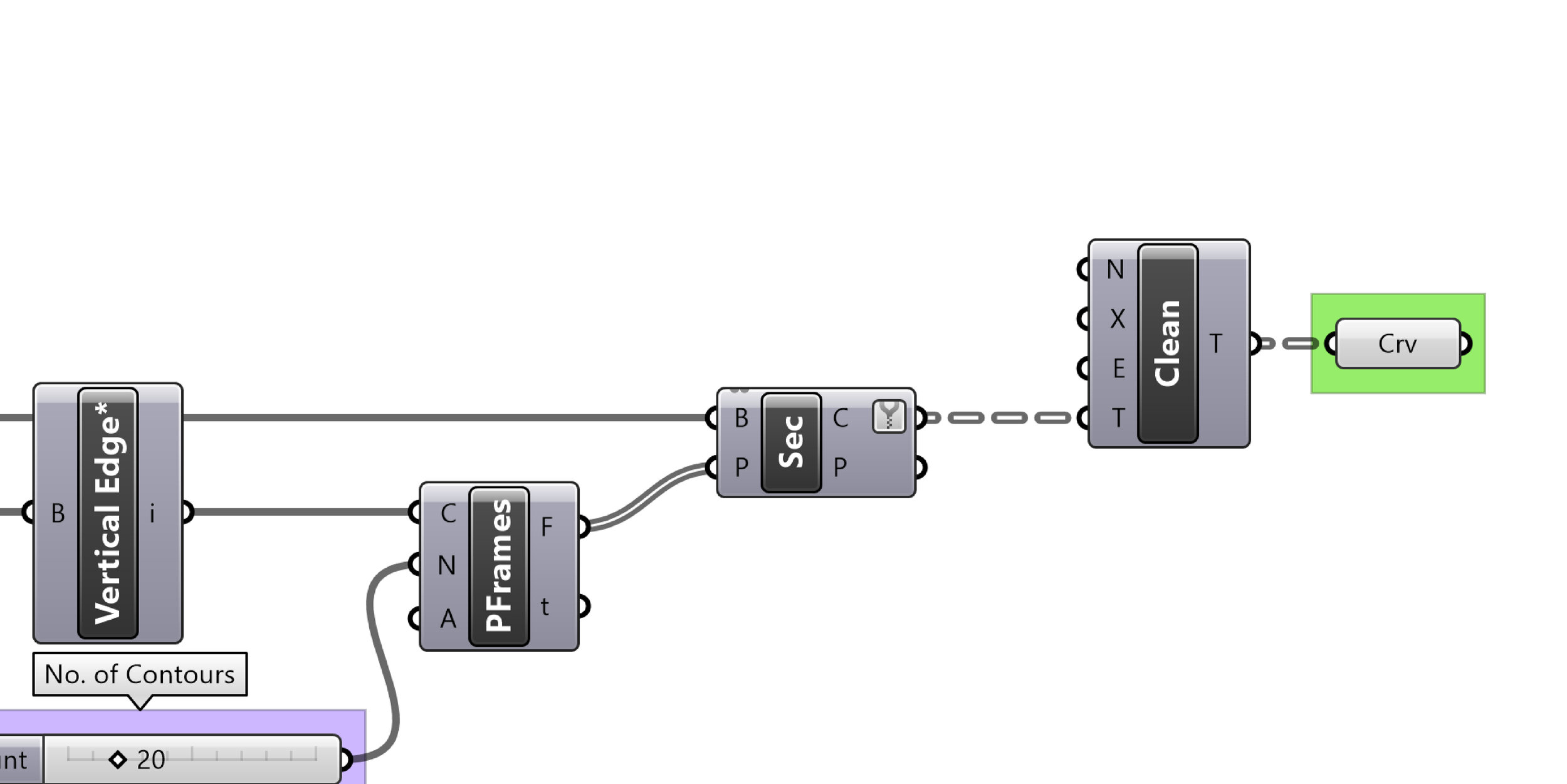
To create a contour of the surface generated in the previous step I first create a single box around the surface using the Bounding Box component. The next step is to find one of the vertical edges of the box and divide the edge by the number of contours we’re after (20 in this example).
The end result of dividing a vertical edge is a series of infinite planes that are going to slice through the geometry and generate curves. To achieve all these steps I’ve used the following components:
Bounding Box > Vertical Edges (see Step 04b) > Perp Frames > Brep | Plane (Sec)
Step 04b*:
The Vertical Edges component in the previous step is a Cluster of components. The Cluster comprises of the following components:
Deconstruct Brep > End Points > Vector 2Pt > Dot Product > Equality > Cull Pattern > List Item
I tend to use Clusters to shorten and tidy up my scripts. It’s important to do this when there aren’t many parameters or inputs needed for this section of the script to run.
Tip #5: Multiple components can be turned into a Cluster by selecting the components first and then clicking on the middle mouse button and choosing the icon which resembles a zipped file (towards the top).
Step 05:
As a final step I’ve used the Clean Tree component to clean up the data generated by the Brep | Plane component. Make sure to click on the E input and set the Boolean to True.
To add colour to these curves, refer to MetaBall Part 02 post.


