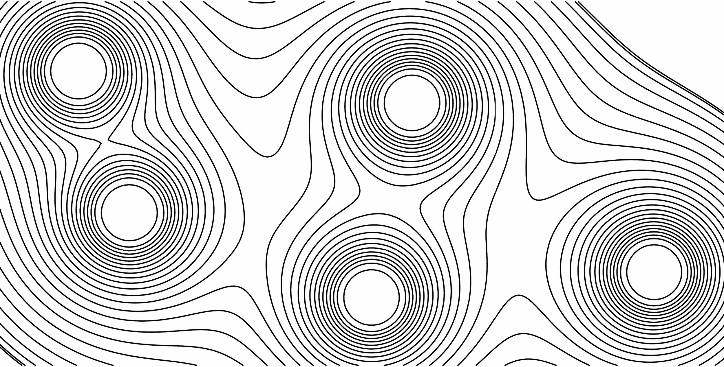
MetaBall Part 01
This post explores the use of Grasshopper’s MetaBall(t) component to produce diagrams. Metaballs are organic-looking n-dimensional isosurfaces, characterised by their ability to meld together when in close proximity to create single, contiguous objects.
MetaBall Part 01 does not require any additional plug-ins for GH. I’m using Rhino 6 and the model units are in mm.
Let’s get started!
Step 00:
The script requires two things to be done in Rhino before moving to GH:
A rough boundary of the area that the MetaBall will be placed inside
A series of points that function as “focal points” to the script
Let’s start by drawing a rectangle 2000 mm long and 1000 mm wide from the Top view (on the xy plane) . The boundary does not need to be a rectangle and can be any type of closed curve. Then place the boundary curve inside a layer called: Crv - Boundary
We also need to draw a series of points that drive the definition. Not all of these points need to be placed inside the boundary curve. Then we place these points inside a layer called: Pt - Focal Point
Step 01:
Now we can start GH and place a MetaBall(t) component on the canvas. The component has four inputs:
P (Points): we feed our Pt - Focal Points her
Pl (Plane): we can ignore this input as long as we stay on the xy plane
T (Threshold): Determines the strength of the MetaBall as well as how the strength is distributed between the focal points
A (Accuracy): Sets the smoothness of the curves generated. The smaller the number, the smoother the curves get in return the script will take longer to run.
Step 02:
To reference the points from Rhino into Grasshopper, I’m going to use the Dynamic Pipeline component. This enables my script to automatically add or deduct the points if there are any changes in Rhino. For this component to work properly, it is crucial to name the layers properly and to make sure the points are placed in the right layer.
Step 03:
By connecting the focal points to the MetaBall(t) component, the colour of the component changes to gray which suggests that the component is running. h
owever, there are no curves generated. This is due to the T input being empty. The most complex part of the script is to calculate and find the right amount for the threshold input.
By examining the T input, we can conclude that it requires relatively small numbers which are tied to the distance between the point and the size of our project. To find the distance between the points, I use the following components (from left to right):
Delaunay Edges (Con) > Length > Bounds > Deconstruct Domain > Maximum
The end result of this chain of components is the maximum distance between the points. Now I can use this number to determine the size of our project which will affect the strength of the T input.
Step 04:
Now we need to define a relationship between the outcome of the previous step and the T input. The relationship needs to produce a smaller number if the distance between the points increases and vice versa. Using the Expression and Series components, I define the relationship as shown on the right-hand side image.
The (1/x)/y formula is an example that I’ve used and it can be replaced by any other formula that resembles similar outcomes.
Step 04b*:
This step is not necessary and it’s function is to control how the strength of the MetaBall(t) is distributed between the focal points. This step will enables us to control the density of the MetaBall curves generated. To do so I used the following components (from left to right):
Bounds > Remap > Graph Mapper > Bounds > Remap
Tip #1: To type some text (0 To 1) use the Panel component. Rather than pressing enter to finish your text, click outside of the yellow canvas.
Tip #2: By right clicking on the Graph Mapper, we can chose a range of graphs to help us edit the data. In my case I used the Bezier option.
Step 05:
Now that the MetaBall(t) component is running, we need to crop the curves generated with our Crv - Boundary which we had set up at the beginning. To do so we need to turn the boundary curve into an extrusion to trim the curves:
Boundary Surface > Unit Z > Extrude
Step 06:
In our final step we use the Trim with Brep component to split the MetaBall curves. TheCi output provides us with the curves that are inside the
Crv - Boundary.


